Gromacs produces graphs in the xmgrace (“xvg”) format. These are simple multi-column data files. The class XVG encapsulates access to such files and adds a number of methods to access the data (as NumPy arrays), compute aggregates, or quickly plot it.
The XVG class is useful beyond reading xvg files. With the array keyword or the XVG.set() method one can load data from an array instead of a file. The array should be simple “NXY” data (typically: first column time or position, further columns scalar observables). The data should be a NumPy numpy.ndarray array a with shape (M, N) where M-1 is the number of observables and N the number of observations, e.g.the number of time points in a time series. a[0] is the time or position and a[1:] the M-1 data columns.
The XVG.error attribute contains the statistical error for each timeseries. It is computed from the standard deviation of the fluctuations from the mean and their correlation time. The parameters for the calculations of the correlation time are set with XVG.set_correlparameters().
See also
The XVG.plot() and XVG.errorbar() methods are set up to produce graphs of multiple columns simultaneously. It is typically assumed that the first column in the selected (sub)array contains the abscissa (“x-axis”) of the graph and all further columns are plotted against the first one.
Plotting from XVG is fairly flexible as one can always pass the columns keyword to select which columns are to be plotted. Assuming that the data contains [t, X1, X2, X3], then one can
plot all observable columns (X1 to X3) against t:
xvg.plot()
plot only X2 against t:
xvg.plot(columns=[0,2])
plot X2 and X3 against t:
xvg.plot(columns=[0,2,3])
plot X1 against X3:
xvg.plot(columns=[2,3])
It is also possible to coarse grain the data for plotting (which typically results in visually smoothing the graph because noise is averaged out).
Currently, two alternative algorithms to produce “coarse grained” (decimated) graphs are implemented and can be selected with the method keyword for the plotting functions in conjuction with maxpoints (the number of points to be plotted):
For simple test data, both approaches give very similar output.
For the special case of periodic data such as angles, one can use the circular mean (“circmean”) to coarse grain. In this case, jumps across the -180º/+180º boundary are added as masked datapoints and no line is drawn across the jump in the plot. (Only works with the simple XVG.plot() method at the moment, errorbars or range plots are not implemented yet.)
See also
In this example we generate a noisy time series of a sine wave. We store the time, the value, and an error. (In a real example, the value might be the mean over multiple observations and the error might be the estimated error of the mean.)
>>> import numpy as np
>>> import gromacs.formats
>>> X = np.linspace(-10,10,50000)
>>> yerr = np.random.randn(len(X))*0.05
>>> data = np.vstack((X, np.sin(X) + yerr, np.random.randn(len(X))*0.05))
>>> xvg = gromacs.formats.XVG(array=data)
Plot value for all time points:
>>> xvg.plot(columns=[0,1], maxpoints=None, color="black", alpha=0.2)
Plot bin-averaged (decimated) data with the errors, over 1000 points:
>>> xvg.errorbar(maxpoints=1000, color="red")
(see output in Figure Plot of Raw vs Decimated data)
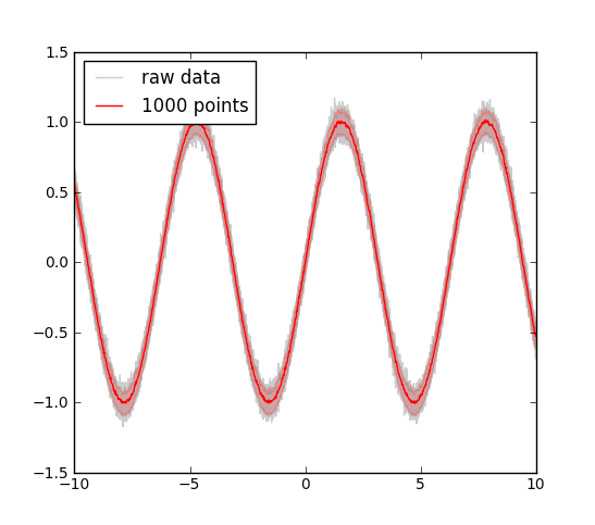
Plot of Raw vs Decimated data. Example of plotting raw data (sine on 50,000 points, gray) versus the decimated graph (reduced to 1000 points, red line). The errors were also decimated and reduced to the errors within the 5% and the 95% percentile. The decimation is carried out by histogramming the data in the desired number of bins and then the data in each bin is reduced by either numpy.mean() (for the value) or scipy.stats.scoreatpercentile() (for errors).
In principle it is possible to use other functions to decimate the data. For XVG.plot(), the method keyword can be changed (see XVG.decimate() for allowed method values). For XVG.errorbar(), the method to reduce the data values (typically column 1) is fixed to “mean” but the errors (typically columns 2 and 3) can also be reduced with error_method = “rms”.
If one wants to show the variation of the raw data together with the decimated and smoothed data then one can plot the percentiles of the deviation from the mean in each bin:
>>> xvg.errorbar(columns=[0,1,1], maxpoints=1000, color="blue", demean=True)
The demean keyword indicates if fluctuations from the mean are regularised [1]. The method XVG.plot_coarsened() automates this approach and can plot coarsened data selected by the columns keyword.
Footnotes
| [1] | When error_method = “percentile” is selected for XVG.errorbar() then demean does not actually force a regularisation of the fluctuations from the mean. Instead, the (symmetric) percentiles are computed on the full data and the error ranges for plotting are directly set to the percentiles. In this way one can easily plot the e.g. 10th-percentile to 90th-percentile band (using keyword percentile = 10). |
Class that represents the numerical data in a grace xvg file.
All data must be numerical. NAN and INF values are supported via python’s float() builtin function.
The array attribute can be used to access the the array once it has been read and parsed. The ma attribute is a numpy masked array (good for plotting).
Conceptually, the file on disk and the XVG instance are considered the same data. Whenever the filename for I/O (XVG.read() and XVG.write()) is changed then the filename associated with the instance is also changed to reflect the association between file and instance.
With the permissive = True flag one can instruct the file reader to skip unparseable lines. In this case the line numbers of the skipped lines are stored in XVG.corrupted_lineno.
A number of attributes are defined to give quick access to simple statistics such as
- mean: mean of all data columns
- std: standard deviation
- min: minimum of data
- max: maximum of data
- error: error on the mean, taking correlation times into account (see also XVG.set_correlparameters())
- tc: correlation time of the data (assuming a simple exponential decay of the fluctuations around the mean)
These attributes are numpy arrays that correspond to the data columns, i.e. :attr:`XVG.array`[1:].
Note
Initialize the class from a xvg file.
| Arguments : |
|
|---|
Represent xvg data as a (cached) numpy array.
The array is returned with column-first indexing, i.e. for a data file with columns X Y1 Y2 Y3 ... the array a will be a[0] = X, a[1] = Y1, ... .
Decimate data a to maxpoints using method.
If a is a 1D array then it is promoted to a (2, N) array where the first column simply contains the index.
If the array contains fewer than maxpoints points or if maxpoints is None then it is returned as it is. The default for maxpoints is 10000.
Valid values for the reduction method:
- “mean”, uses XVG.decimate_mean() to coarse grain by averaging the data in bins along the time axis
- “circmean”, uses XVG.decimate_circmean() to coarse grain by calculating the circular mean of the data in bins along the time axis. Use additional keywords low and high to set the limits. Assumes that the data are in degrees.
- “min” and “max* select the extremum in each bin
- “rms”, uses XVG.decimate_rms() to coarse grain by computing the root mean square sum of the data in bins along the time axis (for averaging standard deviations and errors)
- “percentile” with keyword per: XVG.decimate_percentile() reduces data in each bin to the percentile per
- “smooth”, uses XVG.decimate_smooth() to subsample from a smoothed function (generated with a running average of the coarse graining step size derived from the original number of data points and maxpoints)
| Returns : | numpy array (M', N') from a (M', N) array with M' == M (except when M == 1, see above) and N' <= N (N' is maxpoints). |
|---|
Return data a circmean-decimated on maxpoints.
Histograms each column into maxpoints bins and calculates the weighted circular mean in each bin as the decimated data, using numkit.timeseries.circmean_histogrammed_function(). The coarse grained time in the first column contains the centers of the histogram time.
If a contains <= maxpoints then a is simply returned; otherwise a new array of the same dimensions but with a reduced number of maxpoints points is returned.
Keywords low and high can be used to set the boundaries. By default they are [-pi, +pi].
This method returns a masked array where jumps are flagged by an insertion of a masked point.
Note
Assumes that the first column is time and that the data are in degrees.
Warning
Breaking of arrays only works properly with a two-column array because breaks are only inserted in the x-column (a[0]) where y1 = a[1] has a break.
Return data a error-decimated on maxpoints.
Histograms each column into maxpoints bins and calculates an error estimate in each bin as the decimated data, using numkit.timeseries.error_histogrammed_function(). The coarse grained time in the first column contains the centers of the histogram time.
If a contains <= maxpoints then a is simply returned; otherwise a new array of the same dimensions but with a reduced number of maxpoints points is returned.
See also
Note
Assumes that the first column is time.
Does not work very well because often there are too few datapoints to compute a good autocorrelation function.
Return data a max-decimated on maxpoints.
Histograms each column into maxpoints bins and calculates the maximum in each bin as the decimated data, using numkit.timeseries.max_histogrammed_function(). The coarse grained time in the first column contains the centers of the histogram time.
If a contains <= maxpoints then a is simply returned; otherwise a new array of the same dimensions but with a reduced number of maxpoints points is returned.
Note
Assumes that the first column is time.
Return data a mean-decimated on maxpoints.
Histograms each column into maxpoints bins and calculates the weighted average in each bin as the decimated data, using numkit.timeseries.mean_histogrammed_function(). The coarse grained time in the first column contains the centers of the histogram time.
If a contains <= maxpoints then a is simply returned; otherwise a new array of the same dimensions but with a reduced number of maxpoints points is returned.
Note
Assumes that the first column is time.
Return data a min-decimated on maxpoints.
Histograms each column into maxpoints bins and calculates the minimum in each bin as the decimated data, using numkit.timeseries.min_histogrammed_function(). The coarse grained time in the first column contains the centers of the histogram time.
If a contains <= maxpoints then a is simply returned; otherwise a new array of the same dimensions but with a reduced number of maxpoints points is returned.
Note
Assumes that the first column is time.
Return data a percentile-decimated on maxpoints.
Histograms each column into maxpoints bins and calculates the percentile per in each bin as the decimated data, using numkit.timeseries.percentile_histogrammed_function(). The coarse grained time in the first column contains the centers of the histogram time.
If a contains <= maxpoints then a is simply returned; otherwise a new array of the same dimensions but with a reduced number of maxpoints points is returned.
Note
Assumes that the first column is time.
| Keywords : |
|---|
Return data a rms-decimated on maxpoints.
Histograms each column into maxpoints bins and calculates the root mean square sum in each bin as the decimated data, using numkit.timeseries.rms_histogrammed_function(). The coarse grained time in the first column contains the centers of the histogram time.
If a contains <= maxpoints then a is simply returned; otherwise a new array of the same dimensions but with a reduced number of maxpoints points is returned.
Note
Assumes that the first column is time.
Return smoothed data a decimated on approximately maxpoints points.
If a contains <= maxpoints then a is simply returned; otherwise a new array of the same dimensions but with a reduced number of points (close to maxpoints) is returned.
Note
Assumes that the first column is time (which will never be smoothed/averaged), except when the input array a is 1D and therefore to be assumed to be data at equidistance timepoints.
TODO: - Allow treating the 1st column as data
Default color cycle for XVG.plot_coarsened(): ['black', 'red', 'blue', 'orange', 'magenta', 'cyan', 'yellow', 'brown', 'green']
Default extension of XVG files.
Error on the mean of the data, taking the correlation time into account.
See [FrenkelSmit2002] p526:
error = sqrt(2*tc*acf[0]/T)
where acf() is the autocorrelation function of the fluctuations around the mean, y-<y>, tc is the correlation time, and T the total length of the simulation.
| [FrenkelSmit2002] | D. Frenkel and B. Smit, Understanding Molecular Simulation. Academic Press, San Diego 2002 |
errorbar plot for a single time series with errors.
Set columns keyword to select [x, y, dy] or [x, y, dx, dy], e.g. columns=[0,1,2]. See XVG.plot() for details. Only a single timeseries can be plotted and the user needs to select the appropriate columns with the columns keyword.
By default, the data are decimated (see XVG.plot()) for the default of maxpoints = 10000 by averaging data in maxpoints bins.
x,y,dx,dy data can plotted with error bars in the x- and y-dimension (use filled = False).
For x,y,dy use filled = True to fill the region between y±dy. fill_alpha determines the transparency of the fill color. filled = False will draw lines for the error bars. Additional keywords are passed to pylab.errorbar().
By default, the errors are decimated by plotting the 5% and 95% percentile of the data in each bin. The percentile can be changed with the percentile keyword; e.g. percentile = 1 will plot the 1% and 99% perentile (as will percentile = 99).
The error_method keyword can be used to compute errors as the root mean square sum (error_method = “rms”) across each bin instead of percentiles (“percentile”). The value of the keyword demean is applied to the decimation of error data alone.
See also
XVG.plot() lists keywords common to both methods.
Represent data as a masked array.
The array is returned with column-first indexing, i.e. for a data file with columns X Y1 Y2 Y3 ... the array a will be a[0] = X, a[1] = Y1, ... .
inf and nan are filtered via numpy.isfinite().
Maximum of the data columns.
Aim for plotting around that many points
Mean value of all data columns.
Minimum of the data columns.
Read and cache the file as a numpy array.
Store every stride line of data; if None then the class default is used.
The array is returned with column-first indexing, i.e. for a data file with columns X Y1 Y2 Y3 ... the array a will be a[0] = X, a[1] = Y1, ... .
Plot xvg file data.
The first column of the data is always taken as the abscissa X. Additional columns are plotted as ordinates Y1, Y2, ...
In the special case that there is only a single column then this column is plotted against the index, i.e. (N, Y).
| Keywords : |
|
|---|
Plot data like XVG.plot() with the range of all data shown.
Data are reduced to maxpoints (good results are obtained with low values such as 100) and the actual range of observed data is plotted as a translucent error band around the mean.
Each column in columns (except the abscissa, i.e. the first column) is decimated (with XVG.decimate()) and the range of data is plotted alongside the mean using XVG.errorbar() (see for arguments). Additional arguments:
| Kewords : |
|
|---|
The demean keyword has no effect as it is required to be True.
See also
Read and parse xvg file filename.
Set the array data from a (i.e. completely replace).
No sanity checks at the moment...
Set and change the parameters for calculations with correlation functions.
The parameters persist until explicitly changed.
| Keywords : |
|
|---|
Standard deviation from the mean of all data columns.
Correlation time of the data.
See XVG.error() for details.
Write array to xvg file filename in NXY format.
Note
Only plain files working at the moment, not compressed.
Create a array which masks jumps >= threshold.
Extra points are inserted between two subsequent values whose absolute difference differs by more than threshold (default is pi).
Other can be a secondary array which is also masked according to a.
Returns (a_masked, other_masked) (where other_masked can be None)